Replace outdated snippets in this Old Revision?Yes No
Indice
Scale Likert
Il pacchetto Likert aiuta nella descrizione e nel trattamento delle scale di atteggiamento del tipo Likert.
Gli items devono essere fattori.
Vedi anche:
Pacchetti e dati
library(tidyverse)
library(likert)
data(pisaitems)
Selezioniamo una sola scala come esempio:
items24 <- pisaitems %>%
  select_at(vars(starts_with("ST24Q")))
Per meglio comprendere i risultati, diamo un nome comprensibile agli items della scala:
# nomi degli items
names(items24) <- c(ST24Q01="only if I have to",
                    ST24Q02="one of my favorite hobbies",
                    ST24Q03="like talking about b",
                    ST24Q04="hard to finish b",
                    ST24Q05="happy receving b as a present.",
                    ST24Q06="a waste of time",
                    ST24Q07="enjoy bookstore",
                    ST24Q08="to get information",
                    ST24Q09="cannot sit still and read",
                    ST24Q10="like express opinions about b",
                    ST24Q11="like exchange b")
La funzione likert() organizza i risultati per tutti gli item di una scala:
likert(items24)
##                              Item Strongly disagree Disagree    Agree Strongly agree
## 1               only if I have to          22.82298 35.90570 30.53855      10.732772
## 2      one of my favorite hobbies          20.32308 36.32162 31.93453      11.420770
## 3            like talking about b          21.24927 33.74201 35.96325       9.045464
## 4                hard to finish b          24.95877 40.39249 26.50886       8.139890
## 5  happy receving b as a present.          19.28187 27.65288 40.17350      12.891747
## 6                 a waste of time          42.24040 40.64689 10.97568       6.137024
## 7                 enjoy bookstore          17.84124 33.37107 36.88333      11.904361
## 8              to get information          14.98106 35.41769 35.75990      13.841359
## 9       cannot sit still and read          33.11719 43.12805 16.91875       6.836012
## 10  like express opinions about b          13.53650 27.53867 43.82185      15.102982
## 11                like exchange b          22.51850 33.02265 32.07993      12.378918
Statistiche descrittive
summary(l24)
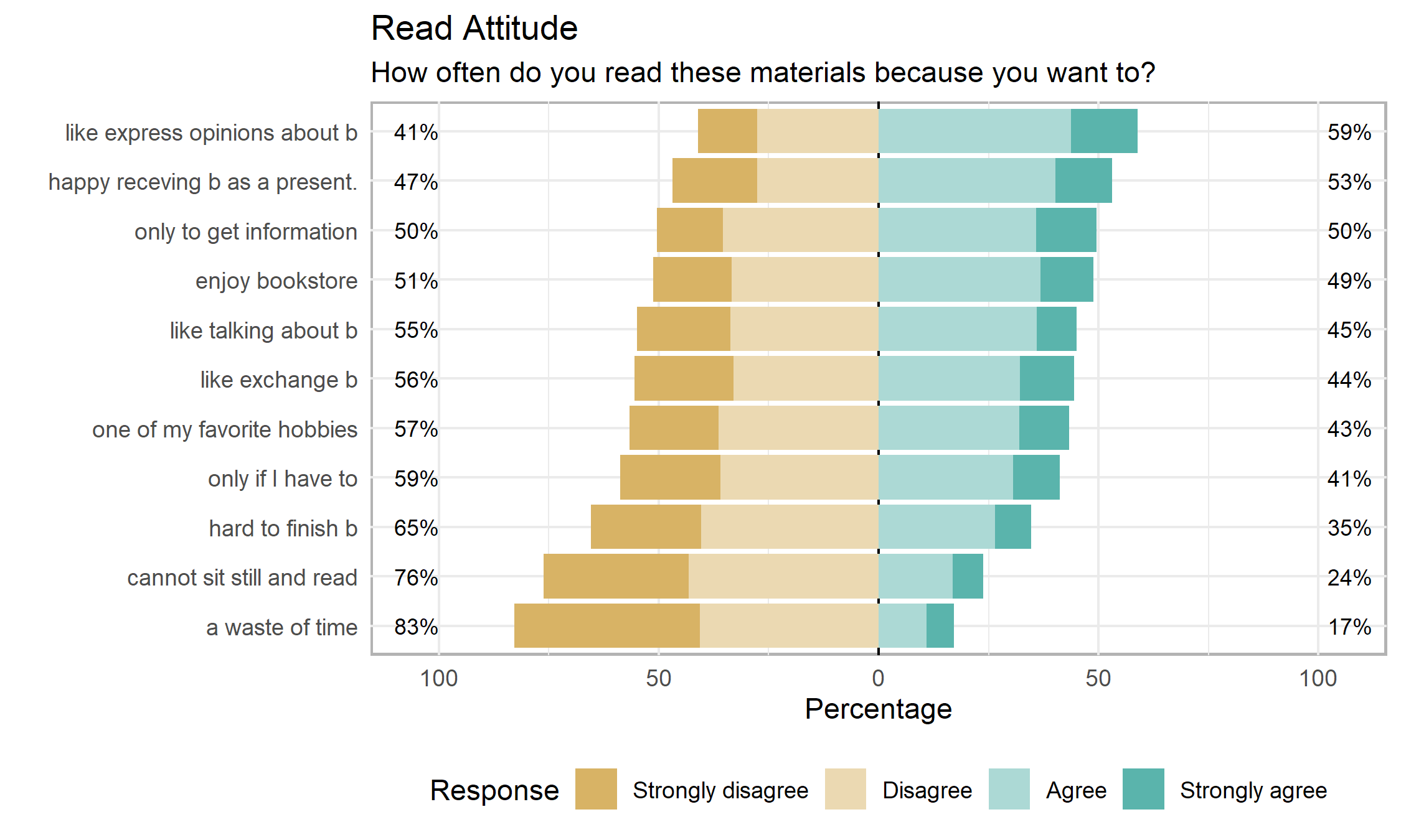
##                              Item      low neutral     high     mean        sd
## 10  like express opinions about b 41.07516       0 58.92484 2.604913 0.9009968
## 5  happy receving b as a present. 46.93475       0 53.06525 2.466751 0.9446590
## 8              to get information 50.39874       0 49.60126 2.484616 0.9089688
## 7                 enjoy bookstore 51.21231       0 48.78769 2.428508 0.9164136
## 3            like talking about b 54.99129       0 45.00871 2.328049 0.9090326
## 11                like exchange b 55.54115       0 44.45885 2.343193 0.9609234
## 2      one of my favorite hobbies 56.64470       0 43.35530 2.344530 0.9277495
## 1               only if I have to 58.72868       0 41.27132 2.291811 0.9369023
## 4                hard to finish b 65.35125       0 34.64875 2.178299 0.8991628
## 9       cannot sit still and read 76.24524       0 23.75476 1.974736 0.8793028
## 6                 a waste of time 82.88729       0 17.11271 1.810093 0.8611554
Il centro (“neutral”) è pari a $(\text{nlevels}-1)/2 + 1$, (in questo caso = 2,5), ma può essere cambiato indicando un valore per l'argomento center, ad esempio:
summary(l24, center = 2)
Di default, gli item vengono ordinati per numero di rispondenti con punteggi alti.
Nota: Gli items “only if I have to”, “hard to finish b(ooks)”, “a waste of time”, “cannot sit still and read” hanno polarità invertita. Vedi Scale Likert: inversione delle polarità
Grafici
Il pacchetto permette di ottenere dei grafici immediatamente utilizzabili per la valutazione delle scale:
plot(l24)
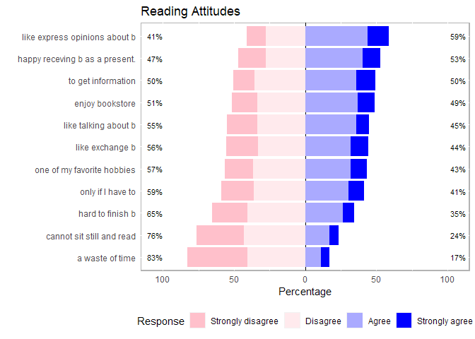
# con colori e titolo
col <- colorRampPalette(c("pink", "white", "blue"))(4)
plot(l24, colors=col) +
  labs(title = "Reading Attitudes")
plot(l24, type='heat', wrap=30, text.size=3.5)

Variabili di raggruppamento
Nella funzione likert() è possibile indicare una variabile di raggruppamento:
l24g <- likert(items24, grouping=pisaitems$CNT)
summary(l24g) %>% head()
##    Group                           Item      low neutral     high     mean        sd
## 1 Canada              only if I have to 60.82666       0 39.17334 2.277647 1.0001779
## 2 Canada     one of my favorite hobbies 61.96628       0 38.03372 2.246538 0.9946381
## 3 Canada           like talking about b 56.91068       0 43.08932 2.274789 0.9467191
## 4 Canada               hard to finish b 71.77194       0 28.22806 2.054269 0.9211851
## 5 Canada happy receving b as a present. 50.13961       0 49.86039 2.384124 0.9730841
## 6 Canada                a waste of time 75.72334       0 24.27666 1.944880 0.9748120
Dal momento che si tratta di un dataframe, possiamo selezionare nell'output le righe che ci interessano:
summary(l24g) %>%
  filter(Group == "Mexico")
##     Group                           Item      low neutral     high     mean        sd
## 1  Mexico              only if I have to 58.64345       0 41.35655 2.273828 0.8912875
## 2  Mexico     one of my favorite hobbies 51.68973       0 48.31027 2.435652 0.8726738
## 3  Mexico           like talking about b 53.23017       0 46.76983 2.372041 0.8832303
## 4  Mexico               hard to finish b 61.01569       0 38.98431 2.258031 0.8783913
## 5  Mexico happy receving b as a present. 42.95741       0 57.04259 2.557262 0.9165585
## 6  Mexico                a waste of time 88.39568       0 11.60432 1.699286 0.7521860
## 7  Mexico                enjoy bookstore 53.62138       0 46.37862 2.385802 0.8478312
## 8  Mexico             to get information 43.57975       0 56.42025 2.605979 0.8836237
## 9  Mexico      cannot sit still and read 76.99317       0 23.00683 1.973779 0.8196108
## 10 Mexico  like express opinions about b 36.67250       0 63.32750 2.689749 0.8728100
## 11 Mexico                like exchange b 51.74623       0 48.25377 2.430137 0.9344254
La funzione non consente di cambiare l'ordinamento per le scale con gruppi, ma è possibile farlo a partire dal risultato:
summary(l24g) %>%
  arrange(Group, desc(high)) %>%
  head()
##    Group                           Item      low neutral     high     mean        sd
## 1 Canada  like express opinions about b 46.59327       0 53.40673 2.495512 0.9272673
## 2 Canada                enjoy bookstore 48.26595       0 51.73405 2.480138 1.0038762
## 3 Canada happy receving b as a present. 50.13961       0 49.86039 2.384124 0.9730841
## 4 Canada           like talking about b 56.91068       0 43.08932 2.274789 0.9467191
## 5 Canada                like exchange b 59.59525       0 40.40475 2.238699 0.9930502
## 6 Canada              only if I have to 60.82666       0 39.17334 2.277647 1.0001779
Vedi le funzioni filter() e arrange()
I grafici:
plot(l24g, group.order=c('Mexico', 'Canada', 'United States'))

Altri esempi sono disponibili nelle demo del pacchetto.
Script di esempio
- es_Likert.R
library(tidyverse)
library(likert)

data(pisaitems)

# selezioniamo una sola scala come esempio
items24 <- pisaitems %>%
  select_at(vars(starts_with("ST24Q")))

# nomi degli items
names(items24) <- c(ST24Q01="only if I have to",
                    ST24Q02="one of my favorite hobbies",
                    ST24Q03="like talking about b",
                    ST24Q04="hard to finish b",
                    ST24Q05="happy receving b as a present.",
                    ST24Q06="a waste of time",
                    ST24Q07="enjoy bookstore",
                    ST24Q08="to get information",
                    ST24Q09="cannot sit still and read",
                    ST24Q10="like express opinions about b",
                    ST24Q11="like exchange b")

likert(items24)

l24 <- likert(items24)
str(l24)

summary(l24)

## # qui non ha senso, perché le alternative sono solo 4
## summary(l24, center = 2)

summary(l24) %>%
  LabRS::kabbit(digits = 2,
                col.names = c("Item", "basso", "neutro", "alto", "media", "sd"),
                caption = "Statistiche riassuntive: output"
                )

plot(l24)

# con colori e titolo
col <- colorRampPalette(c("pink", "white", "blue"))(4)
plot(l24, colors=col) +
  labs(title = "Reading Attitudes")

plot(l24, type='heat', wrap=30, text.size=3.5)

# variabile di raggruppamento
l24g <- likert(items24, grouping=pisaitems$CNT)

summary(l24g) %>% head()

summary(l24g) %>%
  filter(Group == "Mexico")

summary(l24g) %>%
  arrange(Group, desc(high)) %>%
  head()

plot(l24g, group.order=c('Mexico', 'Canada', 'United States'))